
A football team has 65 per cent possession, takes 18 shots and still loses 1–0. Another side has four attempts, scores twice and wins. Fans searching for Manchester City, Nottingham Forest or a Premier League result increasingly see one number beside the score: xG. It is often used to argue that one club deserved more goals, but that is an interpretation, not what the statistic itself proves.
Expected goals measures the quality of shots according to a statistical model built from historical scoring chances. A shot assigned 0.10 xG represents a roughly ten per cent model-estimated probability of becoming a goal under comparable conditions. It does not mean that a player scored one tenth of a goal or that the team is entitled to a goal when enough similar shots accumulate.
The November 2026 Premier League analysis by Opta offered a striking illustration: Nottingham Forest failed to score from 0.86 xG in a defeat at Brentford, while Brentford scored twice from just 0.46 xG. The 2–0 result remains the result. The xG figures help explain why the final score did not describe every attacking opportunity.
What Does xG Mean in Football?
xG stands for expected goals. In a typical shot-based model, each qualifying shot is given a value between zero and one representing the model’s estimated chance that a shot of that type would result in a goal. The shot probabilities for one team can then be added to produce a total expected-goals value for a match.
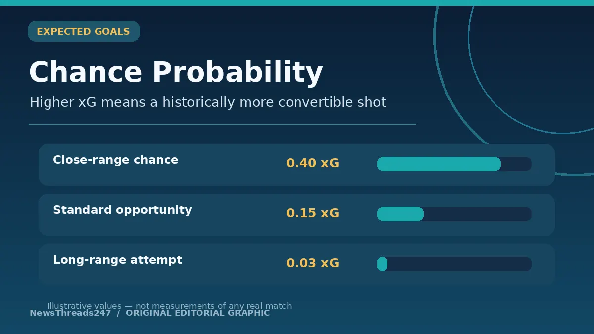
A close-range opportunity from a favorable angle generally receives a higher value than an attempt from far outside the penalty area under pressure. Some models account for the body part used, type of assist, defensive pressure and other shot information. The exact inputs differ among data providers.
The Premier League says its official statistical collection and analysis is handled by Opta. That does not mean every website uses identical xG values. Different models may include different inputs, data quality and treatment of situations, so small differences between providers do not necessarily mean one website is defective.
Imagine a fictional forward taking a shot valued at 0.20 xG. In the model, similar shots would historically convert about one in five times. The forward either scores or does not: the actual outcome is still binary. The 0.20 remains a measure of the pre-shot chance’s estimated quality.
Why Some Shots Are Worth More xG
Distance from goal matters because close shots generally have a better chance of scoring. Angle also matters: a shot from near the byline offers less of the goal to aim at than one from a central position at a comparable distance.
The way the shot arrives can affect its quality. A controlled pass into the penalty area may create a different chance from a bouncing cross or hurried header. Defenders’ positions, a goalkeeper’s angle and whether the attacking player must turn or stretch may also influence the model if those inputs are available.
Not every model incorporates every factor. Some traditional models primarily use shot location, angle and body part, while more advanced approaches may account for defensive pressure or the goalkeeper’s location. The important question when comparing numbers is whose model produced them.
A penalty often receives a relatively high xG value because historically it is converted far more frequently than a distant open-play attempt. That does not guarantee a goal, and the assigned probability may vary by provider. Avoid presenting any one model’s exact figure as universal across all competitions.
A Worked xG Calculation
Suppose a fictional team has three shots. The first is a clear close-range chance valued at 0.40 xG. The second is a more difficult attempt valued at 0.10. The third is a long-range effort worth 0.05. Adding them gives 0.40 + 0.10 + 0.05 = 0.55 xG.
What does 0.55 mean? Under the modeling assumptions, the combined chance values total a little more than half an expected goal. It does not guarantee that the team scores exactly one, nor does it mean the team has a 55 per cent probability of scoring at least once. That latter question requires a different calculation with assumptions about the shots.
If a second team has six shots worth 0.03 each, its xG would be 0.18 despite taking twice as many attempts. This helps explain why the raw shot count can hide the difference between good chances and speculative long-range shooting.
The graphic below uses invented values for teaching. It is not a reproduction of any real player’s performance and should not be used to assess a specific match.
Actual Goals and Expected Goals Are Different
Actual goals decide the scoreboard. Expected goals provides an estimate of chance quality. A team can score three times from 0.7 xG, or fail to score despite creating 2.0 xG. Neither scenario breaks the model. Uncertainty is an essential part of football.
Imagine Team A creates 1.8 xG and scores once; Team B creates 0.6 xG and scores twice. Team B wins 2–1. The analyst can responsibly say Team A created the higher model-estimated volume of chances, but should not say the official score was wrong or that Team A automatically deserved three league points.
This distinction is especially important in emotional match recaps. Fans may say their team was unlucky, the goalkeeper performed unusually well, or the opponents were clinical. Those are plausible interpretations that require looking at the underlying shots and performances rather than repeating only a single xG total.
The November 5 Premier League/Opta analysis described Nottingham Forest scoring six goals from 14.3 xG over its first nine league matches. This is a dated snapshot, not an evergreen statement about the club. It illustrates how a team may generate chances without converting them at a rate close to the model average for a period of time.
How to Calculate Goals Minus xG
A simple comparison subtracts expected goals from actual goals. If a player scores eight goals from 6.5 xG, the difference is +1.5. If the same player scores four from 6.5 xG, the difference is −2.5.
Positive values are often called ‘overperformance’ and negative values ‘underperformance’. They describe the relationship between actual scoring and the model’s expectation, not a conclusive verdict that a player is good or bad at finishing.
A player could outperform xG through excellent finishing, an unusual hot streak, model limitations or a combination. A goalkeeper’s exceptional saves might also suppress an opponent’s goals relative to xG. One match is far too small to settle those explanations.
Compare similar competitions, seasons, opponents and shot totals before making strong claims. A striker who has played 1,800 minutes and accumulated hundreds of touches cannot fairly be compared with a substitute who has taken two shots merely by placing their goals-minus-xG beside each other.
Why xG Does Not Forecast a Match Result
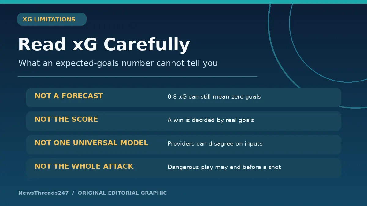
Many people read xG as a probability that a team should win. It is not. Standard xG summarizes shot quality. Match-result probabilities also depend on the opposition, timing, score state, remaining time and other variables.
A team leading 2–0 may defend more deeply and allow the opposition to take shots late in the game. The chasing team can accumulate xG while the leader still wins comfortably. Without the match sequence, the final xG can be misleading.
xG totals may also fail to capture promising attacks that never produce a shot. A player could make a dangerous run and deliver a cross that just misses a teammate; under common shot-based xG definitions, no shot means no xG. The Premier League explicitly notes this limitation.
The current xG figure is also a model output, not a verified physical measurement like the number of goals. Precision to two decimal places can make it look more certain than it really is. Read the figure as an estimate with scope and assumptions.
How xG Differs From Shots on Target
Shots count attempts; shots on target count those that require a save or end in a goal, subject to the competition’s definitions. xG asks about the chance quality of shots, which is a different question. A highly dangerous effort that hits the post can have substantial xG without being registered as a shot on target in some provider datasets.
A team might have five shots on target consisting of weak efforts directed straight at the goalkeeper. Another could have two dangerous chances but only one on target. The first side leads the on-target count, while the second may have the higher xG.
This is why meaningful match analysis uses multiple statistics: possession, territory, shots, shot locations, set pieces, defensive actions and the pattern of chances. The objective is to explain what happened, not find one number that automatically proves a preferred narrative.
Expected Goals Against and Defensive Analysis
xGA means expected goals against: the sum of the estimated quality of shots an opponent created. Teams with low xGA have generally limited opponents to fewer or poorer shots under the model.
Suppose a side concedes only 0.5 xGA in a match but lets in two goals. The defense may have restricted the creation of high-quality chances, but the opponent could have finished unusually well or scored from a low-probability attempt. A deeper look should assess shot locations and goalkeeper responses.
A low xGA across a substantial period can support an argument about defensive performance, but it should be interpreted alongside injuries, opponents and tactics. It is also not identical to the quality of every attacking situation a club prevented before the shot occurred.
The Premier League’s own fantasy glossary distinguishes xG for a player’s or team’s chances from xGA for the chances allowed. Fantasy managers use both because they answer different questions.
Different Providers Can Show Different Numbers
A supporter may notice one app reporting 1.42 xG and another 1.57 for the same match. This can happen because each provider models chance quality differently. A difference of a few hundredths or tenths does not necessarily imply a changed final score or a calculation mistake.
Always name the provider when citing a specific xG total. If comparing several matches or players, use one data source consistently, or explicitly explain why the figures cannot be compared directly.
Models also evolve. Providers may add information about defensive pressure or goalkeeper position and recalibrate their historical probabilities. A 2026 statistic cannot automatically be treated as equivalent to a value collected with a different method a decade earlier.
Strong editorial practice means referring to official league records for actual goals and results while citing the model provider for estimated chance quality. The difference in evidence matters.
Read a Match With a Simple Four-Part Checklist
First, look at the actual result and match state. Who led, when were the goals scored and how much time was left? Second, examine the shot locations and xG values rather than relying on aggregate totals alone.
Third, compare the shot counts with the quality distribution. A team that took 20 distant attempts may have produced less genuine danger than one with four close chances. Fourth, note the model and its limitations, including whether penalties, own goals or situations without shots are treated differently.
Only then draw a proportionate conclusion. ‘This side created higher-quality shooting opportunities’ is often defensible. ‘The wrong team won’ is an opinion rather than a statistical fact.
For readers who want to understand how the actual table is then decided, our football league standings guide explains the separate points and goal-difference rules. xG does not add or remove league points.
Frequently Asked Questions
Is 1.5 xG the same as a 50 per cent chance of scoring?
No. xG totals add shot-level expected values; they do not directly give the probability of scoring at least one goal. That would require a different probability calculation and assumptions.
Can a team win with lower xG?
Yes. Goals decide the result. A team may finish chances efficiently, benefit from a strong goalkeeper or win despite creating fewer high-quality opportunities by the model.
What does a 0.10 xG shot mean?
Under that model, comparable shots historically became goals about ten per cent of the time. The individual attempt still results in either a goal or no goal.
Does xG include every dangerous attack?
Not usually. Common xG models are based on shots; an excellent move ending without a shot may contribute zero xG. The exact treatment varies by provider.
What is the difference between xG and xGA?
xG describes estimated chance quality created by a team or player. xGA describes the estimated quality of shots conceded to opponents.
Sources and Editorial Disclosure
Premier League / Opta, 5 November 2026: Expected Goals v Actual Goals supplies the definition, current example and shot-based limitations. Premier League: Statistics Explained identifies Opta’s official data role. Premier League FPL Glossary explains xG and xGA from a fantasy-football perspective.
All probability examples and the illustrated pitch are hypothetical, not a reconstruction of an actual match. These are original NewsThreads247 editorial diagrams. This explanation does not claim that xG can determine whether a team ‘deserved’ to win or predict an individual match score.